Sklearn at its basic and beginners guide.
Introduction
Scikit-image is a collection of image processing algorithms for the SciPy ecosystem. It has
Pythonic API (written in python), is well documented and aims to provide researchers
and practitioners with well-tested, fundamental building blocks for rapidly constructing
a sophisticated image processing pipelines.
Pythonic API (written in python), is well documented and aims to provide researchers
and practitioners with well-tested, fundamental building blocks for rapidly constructing
a sophisticated image processing pipelines.
It is an open source image processing library for the Python programming language. It includes
algorithms for segmentation, geometric transformations, color space manipulation, analysis, filtering,
morphology, feature detection, and more.
algorithms for segmentation, geometric transformations, color space manipulation, analysis, filtering,
morphology, feature detection, and more.
Scipy image is a part of a large ecosystem of packages and these packages communicate with each other by a common interface which is numpy array. Therefore Scikit-image can be used with
all common packages like matplotlib, pandas etc. As for practical implementation
all common packages like matplotlib, pandas etc. As for practical implementation
The API is used in various industry in the field of medicine, Metallurgy , space imaging etc by
researchers.
researchers.
Now lets get to the implementation.
Images are represented in scikit-image using standard numpy arrays. This allows maximum
interoperability with other libraries in the scientific Python ecosystem, such as matplotlib and scipy.
interoperability with other libraries in the scientific Python ecosystem, such as matplotlib and scipy.
To import Scikit-image we need to use
import skimage
from skimage import data #iit calls all the demo images saved in the package
Example 1
Use numpy to create a image plot .
- import numpy as np
- import matplotlib.pyplot as plt
- %matplotlib inline
- random_image = np.random.random([500, 500])
- plt.imshow(random_image, cmap='gray', interpolation='nearest');
It will plot random noise of image. The black spots are various y n x position generated from
np.random.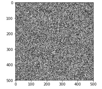
np.random.
Detailed explanation: 1. Numpy is one of the major package in python that helps in many
numerical functions. We use import to call this package so that we can use them in our code.
Also note as np . This is an aliace. Actually used so that we don't have type big names of
packages again an agai. This is a basic python convention that is accepted everywhere.
numerical functions. We use import to call this package so that we can use them in our code.
Also note as np . This is an aliace. Actually used so that we don't have type big names of
packages again an agai. This is a basic python convention that is accepted everywhere.
Other ex would be import pandas as pd, import tensorflow as tf etc.
2. Matplotlib is also another major package that allows plotting capabilities in python. Matplotlib.pyplot
allows to import only pyplot module to the code. This is a common convention when user needs only
a small part of the package and keep the code light.
allows to import only pyplot module to the code. This is a common convention when user needs only
a small part of the package and keep the code light.
3. %matplotlib inline is optional if the code is been written on jupyter notebook and allows showing the
plots in the editor itself.
plots in the editor itself.
4. Now we are using a function from numpy to generate random numbers. It will generate random array of of digits from 1 to 500. Ex [10,34],[43,34] etc.
5. Here we are plotting the image in x-y axis. plt.imshow is a common function that is used to
display image.
display image.
Try to
Example 2
Here we will use submodule of Scikit-image called data which contain bunch of example images.
- from skimage import data
- %matplotlib inline
- import matplotlib.pyplot as plt
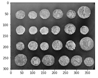
- Coins = data.coins()
- print(type(Coins), Coins.dtype, Coins.shape)
- plt.imshow(coins, cmap='gray', interpolation='nearest');
Detailed explanation: 1. Data module inside skimage contains many demo images that can be used
for practice.
for practice.
4. coins is one of the file. Coins = data.coins(). Here we are storing the coin image inside the Coins
variable.
variable.
5. Here we want to show the type. As said earlier skimage stores image as an array . this will give us
output as numpy.ndarray' and shape as (303, 384
output as numpy.ndarray' and shape as (303, 384
6. Plt.show has the same use as in example 1. Only difference is here we are printing a image. Also
cmap='gray' is giving a grayscale image. Removing this parameter will give a coloured image.
cmap='gray' is giving a grayscale image. Removing this parameter will give a coloured image.
Example 3
Colour images : In Scikit-image color images are a stack of 3d array stacked one over the other.
The last dimension has size 3 and represents the red, green, and blue channels
- from skimage import data
- from matplotlib import pyplot as plt
- %matplotlib inline
- cat = data.chelsea()
- print("Shape:", cat.shape)
- print("Values min/max:", cat.min(), cat.max())
- plt.imshow(cat, interpolation='nearest');

cat[10:110, 10:110, :] = [0, 255, 0] # [red, green, blue]
plt.imshow(cat);
8. cat[10:110, 10:110, :] = [0, 255, 0] # [red, green, blue]
9. plt.imshow(cat);

Detailed explanation: 1,2,3 are explained in example 1,2
4. Chelsie is the file that holds the image cat.
5.here we are printing the shape of the array for the image.
6. Similarly we are printing the minimum and maximum values in array. Here in the output 0 means
black and 255 is pure RGB.
black and 255 is pure RGB.
7. Showing the image
8. Here we are creating a extra element on the image to show how color can be implemented using
an array. Like said earlier the image generated is a numpy array so we can manipulate it adding color
channel in arrays [0, 255, 0] represents red , gree, and blue. By changing them we can different color
to it.
an array. Like said earlier the image generated is a numpy array so we can manipulate it adding color
channel in arrays [0, 255, 0] represents red , gree, and blue. By changing them we can different color
to it.
We can also add 4th dimension also known as alpha layer to the image.
rgba = numpy.concatenate((cat, numpy.zeros((205, 54, 1))), axis=2)
In literature, one finds different conventions for representing image values:
0 - 255 where 0 is black, 255 is white if array holds uint8 datatype
0 - 1 where 0 is black, 1 is white if array holds float datatype
0 - 1 where 0 is black, 1 is white if array holds float datatype
scikit-image supports both conventions--the choice is determined by the data-type of the array.
from skimage import img_as_float, img_as_ubyte
image = data.chelsea()
image_float = img_as_float(image)
image_ubyte = img_as_ubyte(image)
image = data.chelsea()
image_float = img_as_float(image)
image_ubyte = img_as_ubyte(image)
print("type, min, max:", image_float.dtype, image_float.min(), image_float.max())
print("type, min, max:", image_ubyte.dtype, image_ubyte.min(), image_ubyte.max())
print("231/255 =", 231/255.)
print("type, min, max:", image_ubyte.dtype, image_ubyte.min(), image_ubyte.max())
print("231/255 =", 231/255.)
Example 4
In this example we will import images and use them
Since scikit-image operates on NumPy arrays, any image reader library that provides arrays will do.
Options include matplotlib, pillow, imageio, imread, etc.scikit-image conveniently wraps many of
these in the io submodule, and will use whatever option is available:
Options include matplotlib, pillow, imageio, imread, etc.scikit-image conveniently wraps many of
these in the io submodule, and will use whatever option is available:
- from skimage import io
- image = io.imread('../images/img_name.jpg')
- print(type(image))
- print(image.dtype)
- print(image.min(), image.max())
- plt.imshow(image);

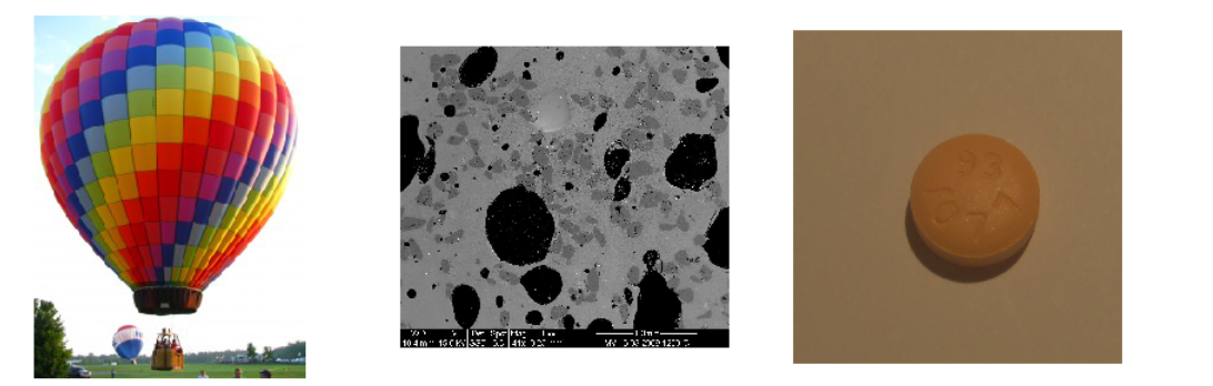
Now if we want to upload multiple files then.
7. ic = io.ImageCollection('../images/*.png:../images/*.jpg')
8. print('Type:', type(ic))
9. Ic.files
8. print('Type:', type(ic))
9. Ic.files
10. f, axes = plt.subplots(nrows=1, ncols=len(ic), figsize=(15, 5))
11. for i, image in enumerate(ic):
axes.flat[i].imshow(image, cmap='gray')
axes.flat[i].axis('off')
Detailed explanation: 1. Here we are using another module io that helps in importing images from
our directory.
our directory.
2. We need to specify the path. In windows we use // to distinguish path while linus / would work
3,4,5 We are trying to print information related to the image. They are self explanatory.
6. Plt.imshow has the same use here just the variable image now has a file taken from the path rather
than from the package.
than from the package.
7. Here there is a little difference. We are calling all the images in a directory. As you may know *.jpg
will look for all images with jpg extension.
will look for all images with jpg extension.
8,9 Ic takes in the file information and print them according to the parameter.
10. We need to now plot not 1 but 3 images. So we are first creating space. Here we select nrows 1
as we want to see them in 1 row but set ncols to length of ic. for example if there are 5 images that
would create 5 columns.
as we want to see them in 1 row but set ncols to length of ic. for example if there are 5 images that
would create 5 columns.
11. Now we print the image 1 by 1 inside a for loop. Here i will run as long as there are files in ic. the
value of i will point the location of the file name and image will take the image 1 by 1.
value of i will point the location of the file name and image will take the image 1 by 1.
For i=0 image will hold the balloon, then the spot and then the pill. It must be remembered that index
in python start from 0 if not mentioned otherwise.
in python start from 0 if not mentioned otherwise.
Example 5
Skimage.io.imshow can only display grayscale and RGB(A) 2D images. By using skimage.io.imshow
we can visualize 2D planes. By fixing one axis, we can observe three different views of the image.
we can visualize 2D planes. By fixing one axis, we can observe three different views of the image.
- %matplotlib inline
- from matplotlib import cm
- from matplotlib import pyplot as plt
- import numpy as np
- from scipy import ndimage as ndi
- from scipy import stats
- data = io.imread("../images/cells.tif")
- print("shape: {}".format(data.shape))
- print("dtype: {}".format(data.dtype))
- print("range: ({}, {})".format(data.min(), data.max()))
12. def show_plane(ax, plane, cmap="gray", title=None):
ax.imshow(plane, cmap=cmap)
ax.set_xticks([])
ax.set_yticks([])
if title:
ax.set_title(title)
_, (a, b, c) = plt.subplots(nrows=1, ncols=3, figsize=(16, 4))
show_plane(a, data[32], title="Plane = 32")
show_plane(b, data[:, 128, :], title="Row = 128")
show_plane(c, data[:, :, 128], title="Column = 128")
show_plane(a, data[32], title="Plane = 32")
show_plane(b, data[:, 128, :], title="Row = 128")
show_plane(c, data[:, :, 128], title="Column = 128")

Detailed explanation: 1-11 are codes that are just extension of what is been done in previous
examples. Here we are using a 2nd package scipy and its modules.
examples. Here we are using a 2nd package scipy and its modules.
12. Def is a keyword in python that is used to create function. A function can hold certain parameters
and can be reused just by passing different values to these parameters.
and can be reused just by passing different values to these parameters.
Now we cant bserve a image in 3d on a 2 d plain. So keeping one axis constant we can view 2 other
axis.
axis.
(a, b, c) = plt.subplots(nrows=1, ncols=3, figsize=(16, 4)) Here we are creating 3 colms to view the
image from 3 direction. Like watching the cube.
image from 3 direction. Like watching the cube.
The fist image is view on top show_plane(a, data[32], title="Plane = 32"). X is kept constant at 32
while y,z is varying. Same is where y is kept constant as 128 and z as 128 resulting in view from 3
sides
while y,z is varying. Same is where y is kept constant as 128 and z as 128 resulting in view from 3
sides
Example 6
Three-dimensional images can be viewed as a series of two-dimensional functions. The display
helper function displays 30 planes of the provided image. By default, every other plane is displayed.
helper function displays 30 planes of the provided image. By default, every other plane is displayed.
import numpy as np
from mpl_toolkits.mplot3d.art3d import Poly3DCollection, Line3DCollection
from scipy import ndimage as ndi
from scipy import stats
import numpy as np
from mpl_toolkits.mplot3d.art3d import Poly3DCollection, Line3DCollection
from scipy import ndimage as ndi
from scipy import stats
import numpy as np
def slice_in_3D(ax, i):
Z = np.array([[0, 0, 0],
[1, 0, 0],
[1, 1, 0],
[0, 1, 0],
[0, 0, 1],
[1, 0, 1],
[1, 1, 1],
[0, 1, 1]])
Z = Z * data.shape
r = [-1,1]
X, Y = np.meshgrid(r, r)
# plot vertices
ax.scatter3D(Z[:, 0], Z[:, 1], Z[:, 2])
# list of sides' polygons of figure
verts = [[Z[0], Z[1], Z[2], Z[3]],
[Z[4], Z[5], Z[6], Z[7]],
[Z[0], Z[1], Z[5], Z[4]],
[Z[2], Z[3], Z[7], Z[6]],
[Z[1], Z[2], Z[6], Z[5]],
[Z[4], Z[7], Z[3], Z[0]],
[Z[2], Z[3], Z[7], Z[6]]]
# plot sides
ax.add_collection3d(
Poly3DCollection(verts, facecolors=(0, 1, 1, 0.25), linewidths=1,
edgecolors='darkblue')
)
verts = np.array([[[0, 0, 0],
[0, 0, 1],
[0, 1, 1],
[0, 1, 0]]])
verts = verts * (60, 256, 256)
verts += [i, 0, 0]
ax.add_collection3d(Poly3DCollection(verts,
facecolors='magenta', linewidths=1, edgecolors='black'))
ax.set_xlabel('plane')
ax.set_ylabel('col')
ax.set_zlabel('row')
# Auto-scale plot axes
scaling = np.array([getattr(ax, 'get_{}lim'.format(dim))() for dim in 'xyz'])
ax.auto_scale_xyz(*[[np.min(scaling), np.max(scaling)]] * 3)
from ipywidgets import interact
def slice_explorer(data, cmap='gray'):
N = len(data)
@interact(plane=(0, N - 1))
def display_slice(plane=34):
fig, ax = plt.subplots(figsize=(20, 5))
ax_3D = fig.add_subplot(133, projection='3d')
show_plane(ax, data[plane], title="Plane {}".format(plane), cmap=cmap)
slice_in_3D(ax_3D, plane)
plt.show()
return display_slice
slice_explorer(data);
def display(im3d, cmap="gray", step=2):
_, axes = plt.subplots(nrows=5, ncols=6, figsize=(16, 14))
vmin = im3d.min()
vmax = im3d.max()
for ax, image in zip(axes.flatten(), im3d[::step]):
ax.imshow(image, cmap=cmap, vmin=vmin, vmax=vmax)
ax.set_xticks([])
ax.set_yticks([])
_, axes = plt.subplots(nrows=5, ncols=6, figsize=(16, 14))
vmin = im3d.min()
vmax = im3d.max()
for ax, image in zip(axes.flatten(), im3d[::step]):
ax.imshow(image, cmap=cmap, vmin=vmin, vmax=vmax)
ax.set_xticks([])
ax.set_yticks([])
display(data)

This will show slice of 3d image in 2d plane
This is a complex version of what we did in the last example.
In the last example we tried to view the image like sides of the cube but how will we view it through.
Detailed explanation:
Mpl_toolkits.mplot3d.art3d is a package that handles 3d models of image. It holds modules to create
a collection of 3D polygons. Now each slice in a array need to be shown
just in np.meshgrid : The function slice_in_3D we are initialize the slides in 3 dimension.
a collection of 3D polygons. Now each slice in a array need to be shown
just in np.meshgrid : The function slice_in_3D we are initialize the slides in 3 dimension.
This function supports both indexing conventions through the indexing keyword argument.
Ax.add_collection3d is creating a 3d box to represent the image and position of the slide in the image.
The overall concept is to create a interactive slides as user sees image one over the other from top.
Slice_explorer function is combining all the input and creating a interactive model. First we are
taking the length on data to create a interactive scroll ( @interact). At the end (def display_slice )
we are also breaking the images to individual slides so we can see them.
def slice_explorer(data, cmap='gray'):
N = len(data)
@interact(plane=(0, N - 1))
def display_slice(plane=34):
fig, ax = plt.subplots(figsize=(20, 5))
ax_3D = fig.add_subplot(133, projection='3d')
show_plane(ax, data[plane], title="Plane {}".format(plane), cmap=cmap)
slice_in_3D(ax_3D, plane)
plt.show()
N = len(data)
@interact(plane=(0, N - 1))
def display_slice(plane=34):
fig, ax = plt.subplots(figsize=(20, 5))
ax_3D = fig.add_subplot(133, projection='3d')
show_plane(ax, data[plane], title="Plane {}".format(plane), cmap=cmap)
slice_in_3D(ax_3D, plane)
plt.show()
Example 7
Now we know how to display images, by Scikik - image we can adjust various properties of it it like
brightness, gama etc.
brightness, gama etc.
Skimage.exposure sub module of Scikik - image contains a number of functions for adjusting image
contrast. These functions operate on pixel values. Generally, image dimensionality or pixel spacing
does not need to be considered.
contrast. These functions operate on pixel values. Generally, image dimensionality or pixel spacing
does not need to be considered.
from scipy import ndimage as ndi
from scipy import stats
from skimage import exposure
from scipy import stats
from skimage import exposure
def plot_hist(ax, data, title=None):
ax.hist(data.ravel(), bins=256)
ax.ticklabel_format(axis="y", style="scientific", scilimits=(0, 0))
if title:
ax.set_title(title)
ax.hist(data.ravel(), bins=256)
ax.ticklabel_format(axis="y", style="scientific", scilimits=(0, 0))
if title:
ax.set_title(title)
gamma_low_val = 0.5
gamma_low = exposure.adjust_gamma(data, gamma=gamma_low_val)
gamma_high_val = 1.5
gamma_high = exposure.adjust_gamma(data, gamma=gamma_high_val)
_, ((a, b, c), (d, e, f)) = plt.subplots(nrows=2, ncols=3, figsize=(12, 8))
show_plane(a, data[32], title="Original")
show_plane(b, gamma_low[32], title="Gamma = {}".format(gamma_low_val))
show_plane(c, gamma_high[32], title="Gamma = {}".format(gamma_high_val))
plot_hist(d, data)
plot_hist(e, gamma_low)
plot_hist(f, gamma_high)
plot_hist(f, gamma_high)
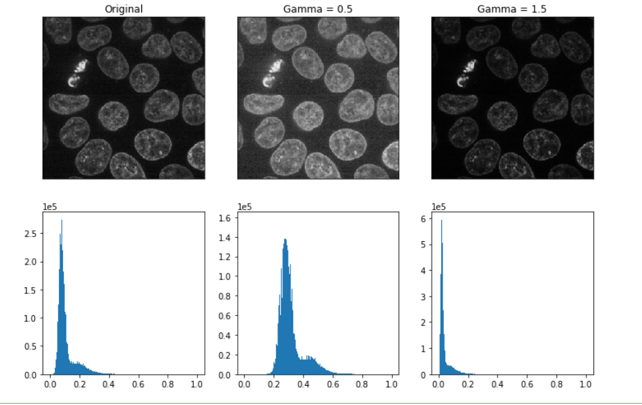
Detailed Explanation: In this code we are trying to enhance the image by skimage module
Exposure. \from skimage import exposure. This module helps us to enhance the properties of image
like brightness, gamma etc. First we are creating a histogram in order to plot the pixel
density. (def plot_his) is taking axis the data of the image and tilt which is none. In the histogram we
are seeing how the increase in gamma is affecting the pixel density. Gama is a log function. Now we
are initializing two gamma levels. .5 and 1.5. Then using exposure.adjust_gamma we are using the
function of exposure module to make changes to the
data file/image gamma_low = exposure.adjust_gamma(data, gamma=gamma_low_val).
Note (a, b, c), (d, e, f) is a tupple, a way of data representation in python
Finally we are showing the changes in the 32 slide from y axis.
Example 8
Edge detection highlights regions in the image where a sharp change in contrast occurs. The intensity
of an edge corresponds to the steepness of the transition from one intensity to another. A gradual
shift from bright to dark intensity results in a dim edge. An abrupt shift results in a bright edge.
of an edge corresponds to the steepness of the transition from one intensity to another. A gradual
shift from bright to dark intensity results in a dim edge. An abrupt shift results in a bright edge.
# copy code from example 7 and then example 8
clipped = exposure.rescale_intensity( data,in_range=(vmin, vmax), out_range=np.float32)
.astype(np.float32)
sobel = np.empty_like( clipped)
for plane, image in enumerate( clipped):
sobel[plane] = filters.sobel(image)
slice_explorer(sobel);

Detailed explanation
The Sobel operator is an edge detection algorithm which approximates the gradient of the image
intensity, and is fast to compute. skimage.filters.sobel has not been adapted for 3D images. It can be
applied planewise to approximate a 3D result. We had used the exposure rescale function to enhance
the image.
Then implemented the function slice_explorer to show the slides with enhanced edges.
intensity, and is fast to compute. skimage.filters.sobel has not been adapted for 3D images. It can be
applied planewise to approximate a 3D result. We had used the exposure rescale function to enhance
the image.
Then implemented the function slice_explorer to show the slides with enhanced edges.
There are many other submodules and API inside Scikit-image . For full list of all the modules please
check thebelow link :
check thebelow link :
http://scikit-image.org/docs/stable/api/api.html
Check the various examples present in http://scikit-image.org/docs/dev/auto_examples/index.html
Reference : wikipidea
Youtube : Image processing in Python.
Comments
Post a Comment